Heat equation

Heat flow, and the corresponding time variation of temperature in ice sheet and glaciers can be described by an advection-diffusion equation, referred to as the heat equation. In cases when melting or freezing is involved is is convenient to instead consider enthalpy (rather than simply heat), but for simiplicity we will initially just consider cases when the ice or snow is below the melting point, so the simpler heat equation is equivelent to an enthalpy formulation.

Below we derive the heat equation from first principles, allowing for temporal and spatial changes in density and velocity. Allowing for these changes results in the same equation that you would reach if you assumed density and velocity constant and uniform, but considering the most general scenario gives us an opportunity to think about the final equation does not depend on if you include them or not.

Setup

We consider a three-dimensional space with cooridinates \(x\), \(y\), and \(z\) corresponding respectively to left-right, in and out of the page, and up and down. Glaciologists often use \(x\) to refer to the glacier direction paralell to the large-scale flow and \(y\) to refer to the across flow direction. We define a small box with side lengths \(\delta x\), \(\delta y\) and \(\delta z\) and volume \(V = \delta x \delta y \delta z\) (Fig. 3). The box contains firn with a mean temperature \(T\) and a mean density \(\rho\). The firn/ice is flowing with a 3-D velocity field defined by the vector field \(\vec{u}\). We ignore the heat content of the air in the pores of the firn and ice.

A note about fields.

Fields are quantities that are defined at every point in space or time. The air temperature in a room can be defined as a field, with every location in the volume of the room associated with a single value: the temperature. Because temperature is a scalar quantity (it requires only one number to represent it at each point in space or time), this field is called a scalar field.

Vector quantities like velocity, displacement, or force, can also be represented in fields. The only difference is that at each location in space or time a vector field has multiple values associated with to represent its vector quantity. For example, a velocity field has components of velocity corresponding to each direction in the coordinate system. In the case of our 3-D cartesian coordinate system, this means that at each point in space and time the velocity field has separate values representing the component of the velocity in the \(x\), \(y\), and \(z\) directions. We will denote these separate components using the glaciological convension of \(u\), \(v\), and \(w\) respectively, and we write \(\vec{u} = (u, v, w)\). It can be a little confusing that the vector field and its x-component are both represented by u’s, but the arrow over the vector field symbol distinguishes it from the x-component of velocity.

It is important to remember that each component, \(u\), \(v\), and \(w\), is potentially a function of \(x\), \(y\), \(z\), or \(t\). In fact, for maximum clarity we could write \(\vec{u}(x,y,z,t) = (u(x,y,z,t), v(x,y,z,t), w(x,y,z,t))\), although we generally do not. As each velocity component is a function of space and time, we can compute space and time gradients of each quantity individually. For example, the \(x\)-derivative of the \(x\)-component of \(\vec{u}\) would be given by \( \frac{\partial u}{\partial x} \) (often called the longitudinal strain rate) or the \(z\)-derivative of the \(z\)-component of \(\vec{u}\) would be given by \( \frac{\partial w}{\partial z} \) (referred to as the across-flow vertical shear stress).

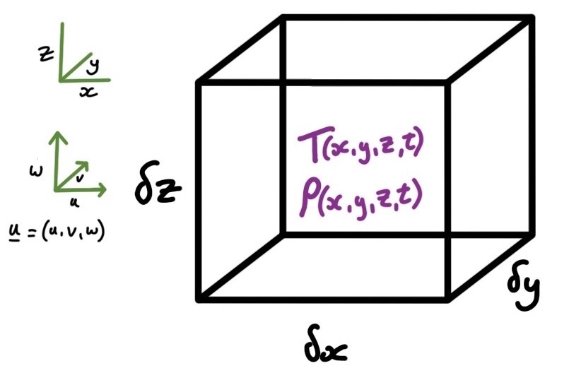
Fig. 3 Consider a small cubic region of space of volume \(V\), filled with firn or ice with a temperature \(T\), a density \(\rho\), and a three-dimensional velocity \(\vec{u}\). The lengths of the sides of the box are \(\delta x\), \(\delta y\) and \(\delta z\) in the \(x\), \(y\) and \(z\) directions respectively.

Advection and diffusion

Heat flows due to two processes: advection and diffusion. Noting the fundamental controls on these two processes help us to guess at what our final heat equation is going to look like.

Advection is the transport of heat due to the flowing ice. For example, if the ice upstream of a given location is warmer, ice flow will move this warmer ice into the location in question and contribute to increasing the temperature. Based just on this intuitive picture of advection, you can guess that the rate at which the temperature changes due to this process is proportional to the velocity of the ice and the rate at which \(T\) increases in an upstream direction. The derivation below proves this intuition correct.

Diffusion is the change in heat content in the box due to spatial variation in conduction. Heat flows from warm areas to cold areas through conduction, at a rate proportoinal to the temperature gradient. So, if the temperature gradient is different in different places, mismatches in the rate of heat conduction leads to areas warming up and cooling down. As we are interested in spatial variations in the temperature gradient, you might guess that the ‘gradient of the gradient of’ the temperature will end up being important. This is called the ‘second-derivative’ or ‘ curvature’ of the temperature, and does indeed appear in our final expression.

Deriving the heat equation

To derive an expression for the rate of change of temperature in this box we equate the rate of change of heat in the box to the rate of heat flow into the box minus the rate of heat flow out of the box. Or, separating the heat flow into contributions from advection and conduction,

(2)\[ \frac{\partial H}{\partial t} = A_{in} - A_{out} + C_{in} - C_{out} \]

where \(H\) is the heat in box, \(A\) and \(C\) are the advective and conductive heat flows and the in and out subscripts denote heat flow in and out. We will also define \(A_{net} = A_{in} - A_{out}\) and \(C_{net} = C_{in} - C_{out}\).

The heat in the box \(H\) is linearly related to the temperature, the density, the volume on the box and the specific heat capacity of ice, \(c\) 2.0 kJ kg\(^{−1}\) K\(^{−1}\):

(3)\[ H = c V \rho T. \]

As a first step we differentiate (3) with respect to \(t\) to expand the left side of (2):

(4)\[ \frac{\partial H}{\partial t} = c V \left(\rho \frac{\partial T}{\partial t} + T \frac{\partial \rho}{\partial t}\right). \]

Next, we derive expressions for all the terms on the right of (2), considering the three direction \(x\), \(y\), and \(z\) in turn.

Advection

We focus first on advective heat flow in the \(x\) direction. Heat advected into the box through its left wall per unit time (per second, say) by advection is

(5)\[ A^x_{in} = u\, \delta y\, \delta z\, c\, \rho\, T \]

where the \(x\) superscript denots that this is in the \(x\)-direction only. To understand this expression, recognize that \(u \delta y \delta z\) is the volume of ice that moves into the box from the left every second (This assumes that the \(x\)-component of the velocity field, \(u\), is positive, if \(u\) was negative \(u \delta y \delta z\) would represent the volume of ice leaving the box, but that’s fine, it would just be a negative heat flux). Also recognize that the heat contained in each cubic meter of ice is given by \(c \rho T\). Therefore the heat entering every second (from the left) is the product of the volume entering every second (\(u \delta y \delta z\)) and the heat contained in each cubic meter (\(c \rho T\)), which gives (5).

To compute the heat advected out of the box through its right wall per second we remember that \(u\), \(\rho\), and \(T\) are all functions of \(x\), \(y\), \(z\), and \(t\). In particular, their \(x\)-dependence is important to us here. We are now considering the right wall of the box, so it is not correct to simply use the same values for \(u\), \(\rho\), and \(T\) as we did above when computing \(A^x_{in}\). Instead we use a trick, which we use in multiple places in this chapters and others, and say that on the right wall these variables take a value that is equal to their values on the left wall plus a small change which depends on their gradient in the \(x\) direction. As noted above we denote their gradients in the \(x\) direction by \( \frac{\partial u}{\partial x} \), \( \frac{\partial \rho}{\partial x} \), and \( \frac{\partial T}{\partial x} \). These tell us how much these variables changes for every meter that you move in the \(x\) direction. In our case, we are moving a distance of \(\delta x\) from one side of the box to the other, so the total change in each variable relative to its values on the left wall of the box is simply \(\delta x \frac{\partial u}{\partial x} \), \(\delta x \frac{\partial \rho}{\partial x} \), and \(\delta x \frac{\partial T}{\partial x} \).

This allows us to write down an expression for \(A^x_{out}\) by repeating the pattern of {eq}A_in1, but replacing the varibles with modified values that include this small change relative to their values on the left wall:

(6)\[ A^x_{out} = \left(u + \delta x \frac{\partial u}{\partial x} \right) \delta y \delta z c \left(\rho + \delta x \frac{\partial \rho}{\partial x} \right) \left(T + \delta x \frac{\partial T}{\partial x}\right). \]

Next we multiple out these brackets to give

(7)\[ A^x_{out} = \delta y \delta z c \left(u \rho T + \delta x \frac{\partial u}{\partial x} \rho T + \delta x u \frac{\partial \rho}{\partial x} T + \delta x u \rho \frac{\partial T}{\partial x} + \delta x^2 \frac{\partial u}{\partial x} \frac{\partial \rho}{\partial x} T + \delta x^2 \frac{\partial u}{\partial x} \rho \frac{\partial T}{\partial x} + \delta x^2 u \frac{\partial \rho}{\partial x} \frac{\partial T}{\partial x} + \delta x^3 \frac{\partial u}{\partial x} \frac{\partial \rho}{\partial x} \frac{\partial T}{\partial x} \right) \]

then omit any terms with \(\delta x\) rasies to a power of 2 or higher, recognizing that \(\delta x\) is already very small so \(\delta x^2\) and \(\delta x^3\) are vanishinglsy small. This leaves

(8)\[ A^x_{out} = \delta y \delta z c \left(u \rho T + \delta x \frac{\partial u}{\partial x} \rho T + \delta x u \frac{\partial \rho}{\partial x} T + \delta x u \rho \frac{\partial T}{\partial x}\right). \]

At this point it is useful to define \(A^x_{net} = A_{in} - A_{out}\) as the net advective heat flow into the box in the \(x\) direction. Using (5) and (8), \(A^x_{net}\) is given by

\[ A^x_{net} = -\delta x \delta y \delta z c \left( \frac{\partial u}{\partial x} \rho T + u \frac{\partial \rho}{\partial x} T + u \rho \frac{\partial T}{\partial x}\right) = - V c \left( \frac{\partial u}{\partial x} \rho T + u \frac{\partial \rho}{\partial x} T + u \rho \frac{\partial T}{\partial x}\right) \]

Using the product rule on the terms containing derivatives of \(u\) and \(\rho\) yields

(9)\[ A^x_{net} = - V c \left( \frac{\partial \left(u \rho\right)}{\partial x} T + u \rho \frac{\partial T}{\partial x}\right) \]

Note

You could simplify this expression further, again using the product rule, to

\[ A^x_{net} = - V c \left( \frac{\partial \left(u \rho T\right)}{\partial x} \right) \]

but leaving it in the form of (9) proves useful for an important step later, which uses mass conservation to simplify the expression.

Equation (9) describes the net advection of heat into the box due to two mechansims. The first term in the parentheses is associated with a change in mass in the box. \( u\rho\) is the mass flux in the \(x\) direction. If this quantity, for example, increased in the \(x\) direction, then mass would be leaving the box over time (because mass would be leaving faster through the right wall than it would be entering through the left wall) and this would be represented by \(\frac{\partial u \rho}{\partial x}\) being larger than zero, which, due to the minus sign in (9), contributes to a decrease in the heat in the box. We will see later that this effect is actually exactly balanced by flow in the other directions or temporal changes in \(\rho\), or both. Therefore, although this term can result in changes in the heat in the box, it does not affect the temperature. We will come back to this point later.

The second term in the parentheses of (9) represents advection resulting from the fact that \(T\) can vary with \(x\). Suppose for example that \(T\) increased with \(x\) and that \(u\) is positive, so there is a component of ice flow along the \(x\) axis in a positive direction. Then ice upstream of our box (at smaller \(x\)) is colder than the ice in the box and this colder ice is being brought into the box by the flow. This contributes to reducing the temperatue in the box and is represented by \(\frac{\partial T}{\partial x} > 0\) and the minus sign on the right of (9).

Applying exactly the same approach to the advective heat fluxes into and out of the box in the \(y\) direction yields:

(10)\[ A^y_{net} = - V c \left( \frac{\partial \left(v \rho\right)}{\partial y} T + v \rho \frac{\partial T}{\partial y}\right). \]

And applying it again in \(z\) direction yields

(11)\[ A^z_{net} = - V c \left( \frac{\partial \left(w \rho\right)}{\partial z} T + w \rho \frac{\partial T}{\partial z}\right). \]

Summing (9), (10), (11) yields an expression for net advective flow

(12)\[ A_{net} = - V c \left[ \left( \frac{\partial \left(u \rho\right)}{\partial x} T + u \rho \frac{\partial T}{\partial x}\right) + \left( \frac{\partial \left(v \rho\right)}{\partial y} T + v \rho \frac{\partial T}{\partial y}\right) + \left( \frac{\partial \left(w \rho\right)}{\partial z} T + w \rho \frac{\partial T}{\partial z}\right) \right] \]

Diffusion

Diffusion of heat is due to spatial gradients in the heat flux due to conduction. In other words, if heat is being conducted through one wall of the box at a different rate than it is being conducted on through the opposite wall, this will contribute to a change in the heat in the box.

Heat conduction is described by Fouriers law of thermal conduction. Applying it in the \(x\) direction gives

(13)\[ q_x = -K\frac{\partial T}{\partial x}, \]

where \(q_x\) is the heat flux in every square meter of cross-sectional area measured perpendicular to the \(x\) axis. The heat conducted into the box through the left wall is therefore

\[ C^x_{in} = -\delta y \delta z K\frac{\partial T}{\partial x}. \]

Because \(K\) and \(\frac{\partial T}{\partial x}\) are functions of \(x\), conduction out of the box through the right wall can be written as

\[ C^x_{out} = -\left(\delta y \delta zK\frac{\partial T}{\partial x} + \delta x \frac{\partial}{\partial x} \left( \delta y \delta z K \frac{\partial T}{\partial x} \right) \right). \]

The net conductive heat flow along hte \(x\) axis is therefore

\[ C^x_{net} = C^x_{in} - C^x_{out} = \delta x \delta y \delta z \frac{\partial}{\partial x} \left( K \frac{\partial T}{\partial x} \right) = V \frac{\partial}{\partial x} \left( K \frac{\partial T}{\partial x} \right) \]

As expected, the second derivative (or ‘curvature’) of the temperature appears in this expression. This can be understood by considering the case when \(K(x) = K\) (i.e. \(K\) is not a function of \(x\)) and therefore

(14)\[ C^x_{net} \propto \frac{\partial^2 T}{\partial x^2}. \]

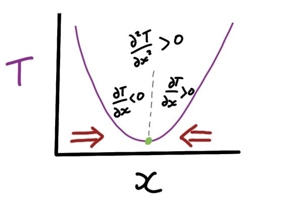
Fig. 4 Schematic of the variation of \(T\) with \(x\) in the region of a minimum in \(T\). As indicated on the plot, the gradient of \(T\) is negative to the left and positive to the right of the minimum. This causes heat to flow towards the minimum, as indicated by the large red arrows.

Consider a location with a local minimum in \(T\) (Fig. 4). Immediately to the left of this location \(\frac{\partial T}{\partial x} < 0\). Immediately to the right, \(\frac{\partial T}{\partial x} > 0\) - \(\frac{\partial T}{\partial x}\) is increasing with \(x\). In other words, \(\frac{\partial^2 T}{\partial x^2} > 0\), so according to (14) this process contributes to an increase in heat in this location, reducing the depth of the minima. This makes sense because we are at a minimum in \(T\), so in both directions higher \(T\) causes heat to be conducted towards this minimum. The same argument applies, not just at minima (or in reverse at maxima) in \(T\), but anywhere with curvature in \(T\): its all down to the gradient in \(T\) being different on side of a given location than it is on the other side, so that the net contribution of conduction is to either increase or decrease tempeature.

Applying the same approach outlined above to in the \(y\) and \(z\) directions gives us

(15)\[ C^y_{net}= V \frac{\partial}{\partial y} \left( K \frac{\partial T}{\partial y} \right) \]

and

(16)\[ C^z_{net} = V \frac{\partial}{\partial z} \left( K \frac{\partial T}{\partial z} \right) \]

Bringing everything together

Bringing together expressions for the net advective flow, \(A_{net}\) ((12)), the net conductive heat flows in each direction, ((14), (15), (16)), and the rate of change of heat in the box ((4)) gives us

(17)\[ c \left(\rho \frac{\partial T}{\partial t} + T \frac{\partial \rho}{\partial t}\right)= - c \left[ \left( \frac{\partial \left(u \rho\right)}{\partial x} T + u \rho \frac{\partial T}{\partial x}\right) + \left( \frac{\partial \left(v \rho\right)}{\partial y} T + v \rho \frac{\partial T}{\partial y}\right) + \left( \frac{\partial \left(w \rho\right)}{\partial z} T + w \rho \frac{\partial T}{\partial z}\right) \right] + \frac{\partial}{\partial x} \left( K \frac{\partial T}{\partial x} \right) + \frac{\partial}{\partial y} \left( K \frac{\partial T}{\partial y} \right) + \frac{\partial}{\partial z} \left( K \frac{\partial T}{\partial z} \right) \]

Notice that the volume of the box \(V\) has cancelled from both sides of this expression. Let’s think about what this cancelling of \(V\) really means. \(V\) appeared on the left of this expression because it takes more heat to increase the temperature of a larger box than a smaller box. \(V\) appeared on the right of this expression because all the heat fluxes into and out of the box for given \(T\), \(\vec{u}\) and \(\rho\) fields, are larger for a larger box than a smaller one because the walls are larger. This explains what \(V\) cancelling means: It takes more heat to change the temperature of a larger box, but a larger box gets more heat from set of conditions. It also makes a lot of sense that \(V\) should cancel because the size and shape this box was chosen arbitrarily and for convenience and should not appear in our final result. In fact, the expression above is very close to our final result. However, there is one interesting simplification that remains to be made.

Mass conservation

To apply the principle of mass conservation to our box, we will apply the same approach as we did above. We define the mass in the box as \(M = V \rho\), and differentiate to get

\[ \frac{\partial M}{\partial t} = V \frac{\partial \rho}{\partial t}. \]

Note the \(V\) is constant in time so it is unaffected by the differentiation. We equate this to the net rate of mass flow it to the box through the walls.

(18)\[ V \frac{\partial \rho}{\partial t} = M_{net}. \]

Next we write down expressions for the rate of mass flow in and out through each wall of the box, considering each direction in turn. The mass flowing in through the left wall in the \(x\) direction is

\[ M^x_{in} = \delta y \delta z \rho u \]

and the mass flowing out through the right wall is

\[ M^x_{out} = \delta y \delta z \left(\rho u + \delta x \frac{\partial \left(u \rho \right)}{\partial x}\right). \]

Therefore the net mass flow in this direction is

\[ M^x_{net} = M^x_{in} - M^x_{out} = -\delta y \delta z \delta x \frac{\partial \left(u \rho \right)}{\partial x} = -V \frac{\partial \left(u\rho \right)}{\partial x}. \]

Applying the same approach in the other directions and combining the results with the expression above gives us the net rate of mass input to the box,

\[ M_{net} = -V \left(\frac{\partial \left(u \rho \right)}{\partial x} + \frac{\partial \left(v \rho \right)}{\partial y} + \frac{\partial \left(w\rho \right)}{\partial z} \right). \]

which we can combine with (18) to give

(19)\[ \frac{\partial \rho}{\partial t} = - \left(\frac{\partial \left(u\rho \right)}{\partial x} + \frac{\partial \left(v\rho \right)}{\partial y} + \frac{\partial \left(w \rho \right)}{\partial z} \right) \]

This is a general statement of mass conservation. It says that the flux divergence is the negative of densification. For those familiar with the notation, it can be expressed more compactly as

\[ \dot{\rho} = \vec{\nabla} \cdot \vec{q} \]

where \(\vec{q} \) is the flux, \( \vec{q}= \vec{u} \rho\), and \(\vec{\nabla}\) is the del operator, \(\vec{\nabla} = \vec{i}\frac{\partial }{\partial x} + \vec{j} \frac{\partial }{\partial y}+ \vec{k}\frac{\partial }{\partial z}. \)

Equation (19) can be understood by considering a simply scenario where \(\rho\) is uniform in space but can change in time, and ice flow is along the \(z\) axis, \(\vec{u} = w\). Under these conditions (19) reduces to

(20)\[ \frac{\partial \rho}{\partial t} = - \rho \frac{\partial w }{\partial z} \]

Consider the case when \(w\) increases with \(w\). The ice above any given location is flowing faster than the ice below, leading to vertical stretching. As expected, according to (20), stretching is associated with a reduction in density. The reverse is also intuitive. If \(w\) decreases with \(x\), ice above any given location is flowing faster than the ice below, leading to vertical compression. It makes sense that, (20) says this is is associated with densification. In fact, this is a common situation in the relatively low density, near-surface layer of the ice sheets called firn.

Substituting in (19) to (17) gives us

(21)\[ \frac{\partial T}{\partial t} = - u \frac{\partial T}{\partial x} - v \frac{\partial T}{\partial y} - w \frac{\partial T}{\partial z} + \frac{1}{c \rho}\left[\frac{\partial}{\partial x} \left( K \frac{\partial T}{\partial x} \right) + \frac{\partial}{\partial y} \left( K \frac{\partial T}{\partial y} \right) + \frac{\partial}{\partial z} \left( K \frac{\partial T}{\partial z} \right)\right] \]

Again, for those familiar with the notation, a more compact way to write this is with the del operator:

\[ \frac{\partial T}{\partial t} = -\vec{u} \cdot \vec{\nabla}T + \frac{1}{c \rho} \vec{\nabla} \cdot K \vec{\nabla}T. \]

Let’s note what happened here: the tern on the right of (17), \( c T \frac{\partial \rho}{\partial t}\), representing the heat density, i.e. how much heat is in each cubic meter, cancelled with the three flux diveregence terms on the right (\(c T \frac{\partial \left(u\rho \right)}{\partial x}\) etc.). This shows us that while these divergence terms can change the ammount of heat in the box, they cannot change the temperature because the density in the box changes to counterbalance any change in the heat content. For example, suppose that spatial gradients in flux caused the heat content in the box to double. At the same time, the density in the box would also double, meaning that the ice requires double the heat to maintain the same temperatue as it had before the change.

Equation (21) is our final complete form of the heat equation that we will analyze in the following pages.