The gradient of Antarctic Ice Sheet

As an aside, in this section we use the concept of gradient introduced on the previous page to compute the slope of the Antarctic Ice SHeet using some surface elevation data.

In this section we will:

• load the bedmachine dataset from a version stored in the cloud

• computes the surface gradient in the \(x\) and \(y\) directions

• computes the slope from these two components

1. Import packages

We will import packages required for opening the data (fsspec), doing computations (numpy), storing the data and results in memory and plotting them (xarray), and plotting with interactive features (hvplot.xarray).

import fsspec
import numpy as np
import xarray as xr
import hvplot.xarray

2. Lazily load the data

First we get a ‘mapper’ which points to the data in cloud storage, then we lazily load it in to a multi-dimensional array called an xarray, which we cam bm.

bm_mapper = fsspec.get_mapper('gs://ldeo-glaciology/bedmachine/bm.zarr', mode='ab')
bm = xr.open_zarr(bm_mapper)  

Let’s take a look at the xarray we get from the cell above

bm

<xarray.Dataset>
Dimensions:    (y: 13333, x: 13333)
Coordinates:
  * x          (x) int32 -3333000 -3332500 -3332000 ... 3332000 3332500 3333000
  * y          (y) int32 3333000 3332500 3332000 ... -3332000 -3332500 -3333000
Data variables:
    bed        (y, x) float32 dask.array<chunksize=(3000, 3000), meta=np.ndarray>
    errbed     (y, x) float32 dask.array<chunksize=(3000, 3000), meta=np.ndarray>
    firn       (y, x) float32 dask.array<chunksize=(3000, 3000), meta=np.ndarray>
    geoid      (y, x) int16 dask.array<chunksize=(3000, 3000), meta=np.ndarray>
    mask       (y, x) int8 dask.array<chunksize=(3000, 3000), meta=np.ndarray>
    source     (y, x) int8 dask.array<chunksize=(3000, 3000), meta=np.ndarray>
    surface    (y, x) float32 dask.array<chunksize=(3000, 3000), meta=np.ndarray>
    thickness  (y, x) float32 dask.array<chunksize=(3000, 3000), meta=np.ndarray>
Attributes: (12/25)
    Author:                                 Mathieu Morlighem
    Conventions:                            CF-1.7
    Data_citation:                          Morlighem M. et al., (2019), Deep...
    Notes:                                  Data processed at the Department ...
    Projection:                             Polar Stereographic South (71S,0E)
    Title:                                  BedMachine Antarctica
    ...                                     ...
    spacing:                                [500]
    standard_parallel:                      [-71.0]
    straight_vertical_longitude_from_pole:  [0.0]
    version:                                05-Nov-2019 (v1.38)
    xmin:                                   [-3333000]
    ymax:                                   [3333000]

xarray.Dataset

• Dimensions:
  • y: 13333
  • x: 13333
• Coordinates: (2)
  • x
    (x)
    int32
    -3333000 -3332500 ... 3333000

    long_name :

    Cartesian x-coordinate

    standard_name :

    projection_x_coordinate

    units :

    meter

    array([-3333000, -3332500, -3332000, ...,  3332000,  3332500,  3333000],
          dtype=int32)

  • y
    (y)
    int32
    3333000 3332500 ... -3333000

    long_name :

    Cartesian y-coordinate

    standard_name :

    projection_y_coordinate

    units :

    meter

    array([ 3333000,  3332500,  3332000, ..., -3332000, -3332500, -3333000],
          dtype=int32)

• Data variables: (8)
  • bed
    (y, x)
    float32
    dask.array<chunksize=(3000, 3000), meta=np.ndarray>

    grid_mapping :

    mapping

    long_name :

    bed topography

    source :

    IBCSO and Mathieu Morlighem

    standard_name :

    bedrock_altitude

    units :

    meters

    Array Chunk Bytes 678.13 MiB 34.33 MiB Shape (13333, 13333) (3000, 3000) Count 2 Graph Layers 25 Chunks Type float32 numpy.ndarray

  • errbed
    (y, x)
    float32
    dask.array<chunksize=(3000, 3000), meta=np.ndarray>

    grid_mapping :

    mapping

    long_name :

    bed topography/ice thickness error

    source :

    Mathieu Morlighem

    units :

    meters

    Array Chunk Bytes 678.13 MiB 34.33 MiB Shape (13333, 13333) (3000, 3000) Count 2 Graph Layers 25 Chunks Type float32 numpy.ndarray

  • firn
    (y, x)
    float32
    dask.array<chunksize=(3000, 3000), meta=np.ndarray>

    grid_mapping :

    mapping

    long_name :

    firn air content

    source :

    FAC model from Ligtenberg et al., 2011, forced by RACMO2.3p2 (van Wessem et al., 2018)

    units :

    meters

    Array Chunk Bytes 678.13 MiB 34.33 MiB Shape (13333, 13333) (3000, 3000) Count 2 Graph Layers 25 Chunks Type float32 numpy.ndarray

  • geoid
    (y, x)
    int16
    dask.array<chunksize=(3000, 3000), meta=np.ndarray>

    geoid :

    eigen-6c4 (Forste et al 2014)

    grid_mapping :

    mapping

    long_name :

    EIGEN-EC4 Geoid - WGS84 Ellipsoid difference

    standard_name :

    geoid_height_above_reference_ellipsoid

    units :

    meters

    Array Chunk Bytes 339.07 MiB 17.17 MiB Shape (13333, 13333) (3000, 3000) Count 2 Graph Layers 25 Chunks Type int16 numpy.ndarray

  • mask
    (y, x)
    int8
    dask.array<chunksize=(3000, 3000), meta=np.ndarray>

    flag_meanings :

    ocean ice_free_land grounded_ice floating_ice lake_vostok

    flag_values :

    [0, 1, 2, 3, 4]

    grid_mapping :

    mapping

    long_name :

    mask

    source :

    Antarctic Digital Database (rock outcrop) and Jeremie Mouginot (pers. comm., grounding lines)

    valid_range :

    [0, 4]

    Array Chunk Bytes 169.53 MiB 8.58 MiB Shape (13333, 13333) (3000, 3000) Count 2 Graph Layers 25 Chunks Type int8 numpy.ndarray

  • source
    (y, x)
    int8
    dask.array<chunksize=(3000, 3000), meta=np.ndarray>

    flag_meanings :

    REMA_IBCSO mass_conservation interpolation hydrostatic streamline_diffusion gravity seismic multibeam

    flag_values :

    [1, 2, 3, 4, 5, 6, 7, 10]

    grid_mapping :

    mapping

    long_name :

    data source

    source :

    Mathieu Morlighem

    valid_range :

    [1, 10]

    Array Chunk Bytes 169.53 MiB 8.58 MiB Shape (13333, 13333) (3000, 3000) Count 2 Graph Layers 25 Chunks Type int8 numpy.ndarray

  • surface
    (y, x)
    float32
    dask.array<chunksize=(3000, 3000), meta=np.ndarray>

    grid_mapping :

    mapping

    long_name :

    ice surface elevation

    source :

    REMA (Byrd Polar and Climate Research Center and the Polar Geospatial Center)

    standard_name :

    surface_altitude

    units :

    meters

    Array Chunk Bytes 678.13 MiB 34.33 MiB Shape (13333, 13333) (3000, 3000) Count 2 Graph Layers 25 Chunks Type float32 numpy.ndarray

  • thickness
    (y, x)
    float32
    dask.array<chunksize=(3000, 3000), meta=np.ndarray>

    grid_mapping :

    mapping

    long_name :

    ice thickness

    source :

    Mathieu Morlighem

    standard_name :

    land_ice_thickness

    units :

    meters

    Array Chunk Bytes 678.13 MiB 34.33 MiB Shape (13333, 13333) (3000, 3000) Count 2 Graph Layers 25 Chunks Type float32 numpy.ndarray

• Attributes: (25)

  Author :

  Mathieu Morlighem

  Conventions :

  CF-1.7

  Data_citation :

  Morlighem M. et al., (2019), Deep glacial troughs and stabilizing ridges unveiled beneath the margins of the Antarctic ice sheet, Nature Geoscience (accepted)

  Notes :

  Data processed at the Department of Earth System Science, University of California, Irvine

  Projection :

  Polar Stereographic South (71S,0E)

  Title :

  BedMachine Antarctica

  false_easting :

  [0.0]

  false_northing :

  [0.0]

  grid_mapping_name :

  polar_stereographic

  ice_density (kg m-3) :

  [917.0]

  inverse_flattening :

  [298.2794050428205]

  latitude_of_projection_origin :

  [-90.0]

  license :

  No restrictions on access or use

  no_data :

  [-9999.0]

  nx :

  [13333.0]

  ny :

  [13333.0]

  proj4 :

  +init=epsg:3031

  sea_water_density (kg m-3) :

  [1027.0]

  semi_major_axis :

  [6378273.0]

  spacing :

  [500]

  standard_parallel :

  [-71.0]

  straight_vertical_longitude_from_pole :

  [0.0]

  version :

  05-Nov-2019 (v1.38)

  xmin :

  [-3333000]

  ymax :

  [3333000]

3. Compute the two components of the gradient

We will use the numpy function numpy.gradient The second argument is the grid spacing, which is the same in both directions in this case. It is stored in the attributes of the xarray (and were loaded from the zarr in cloud storage).

dhdy, dhdx = np.gradient(bm.surface.values,bm.attrs['nx'][0])

4. Compute the slope by taking the pythagorean sum of the two components.

\[ S = \sqrt{\left(\frac{\partial h}{\partial x}\right)^2 + \left(\frac{\partial h}{\partial y}\right)^2} \]

and add this to the xarray as a new field. Also define a name and units for the new field.

slope = xr.zeros_like(bm.thickness)
slope.values = np.sqrt(dhdy**2 + dhdx**2)
bm['slope'] = slope
bm.slope.attrs['long_name'] = 'ice surface slope'
bm.slope.attrs['units'] = '-'

5. Plotting

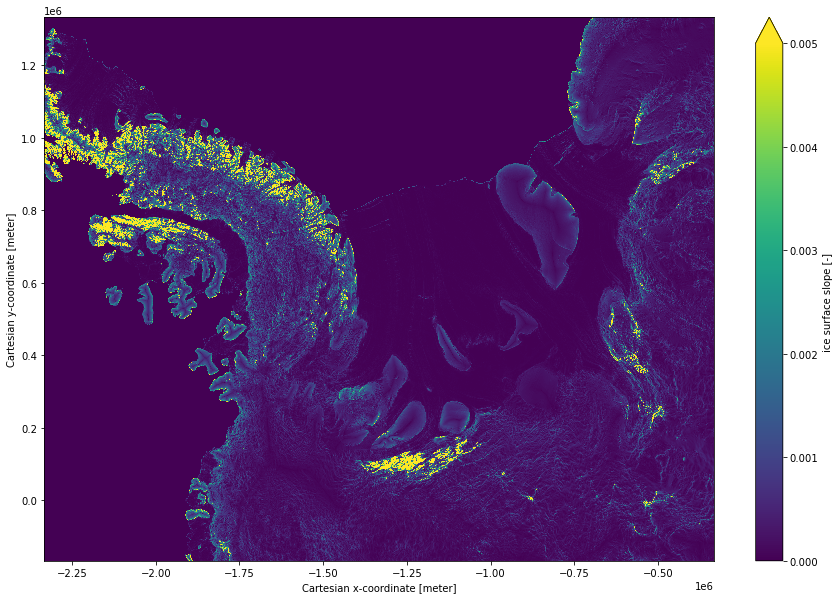
Let’s plot a subset of the slopes to examine the orderof magnitude of the slopes.

subset_of_slope = bm.slope.isel(x = slice(2000,3000), y = slice(4000,5000))

options = dict(x = 'x', y = 'y', clim = (0, 0.001), width = 800, height = 800, cmap = 'viridis')

subset_of_slope.hvplot(**options);

bm.slope.isel(x = slice(2000,6000), y = slice(4000,7000)).plot(vmin = 0, vmax = 0.005, size = 10);

all_slope_coarse = bm.slope.coarsen(x=5,y=5,boundary='trim').mean().persist()
options = dict(x='x', y='y', clim=(0, 0.001), width=800, height=800, cmap='viridis')
all_slope_coarse.hvplot(**options)